

Nonlinear Regression
Get wiggly.

In this week’s article, we learn how to fit nonlinear models.
Is Simplicity Best?
Last week, we calculated the closed-form equation for a simple linear model, but how do we fit a regression model if our system is more complicated than a line?
To begin, we can look at the output of a simple linear regression model where the independent variable is time and the dependent variable is the log-transformed price of the S&P 500 cash index (SPX). Note that we are claiming that time is causing price to act a certain way and not the other way around, that price depends on time.
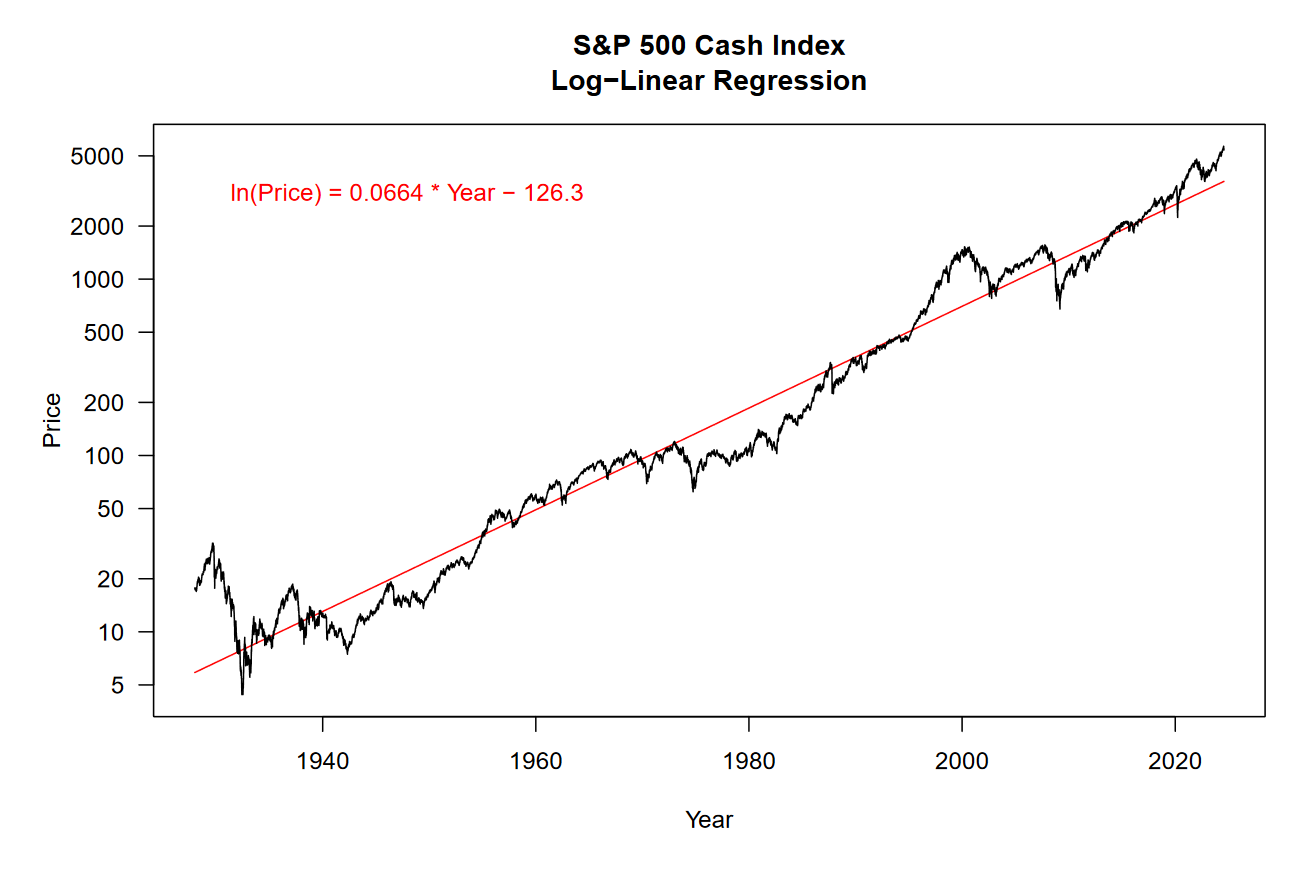
Even a single line can explain most of the variation seen in the price of the SPX.
Take a peek at the equation in the top-left corner of the plot, this is the output of our model. Using this equation, you can plug in any year and get an approximate log price for the S&P 500.
If you look at the y-axis, it’s apparent that this is not a linear scale. We are viewing the data on a log-scale, and this is the same scale that our model was fit on. Because compounding returns grow exponentially, we have to take the logarithm of price for its relationship to time to appear linear.
Goodness of Fit
While you might have intuitively noticed that our model fits the data well, we have a couple of metrics that quantify just how well it fits. These are called “goodness-of-fit” measures. These metrics are calculated before the model output is transformed back to standard units.
First, we will look at the coefficient of determination (also known as R², pronounced “R squared”). This is the squared correlation between our data and the model prediction. For the above model, we have an R² value of 96.22%, meaning that our model explains 96.22% of the variation in the log price of the SPX.
Our next measure is the root mean squared deviation (RMSD). This is calculated by taking the difference between paired data points, squaring those deviations, summing the squared values, and finally taking the square root of that sum. This value is 0.3666 for the above model.
Think of the RMSD as a measure that we want to minimize. The smaller it is, the better our model fits the data. This is the main principle behind using an optimizer to fit our models, which we will discuss in the next section.
Optimization
Mathematical optimization attempts to either minimize or maximize the output for a given function. This is an oversimplification, but it will suffice.
We can use an analogy to understand what an optimizer is trying to do.
Imagine you are standing out in a field. Your job is to try to get as high up as possible (maximize your elevation). You see a hill nearby and start walking up it. It’s seems to be working, you are steadily gaining elevation!
Once you reach the top of the hill, there’s nothing near you that you can keep climbing. Even if you notice a bigger hill out in the distance, that would require you decrease your elevation before it will rise again.
Essentially, you have done what most simple optimizers can do. To the best of your ability, you increased your elevation but maybe you ended up on a smaller hill than what was possible.
Translating the analogy over to an actual algorithm: our optimizer will be fitting a general form of a model by which it will try to minimize the sum of squared deviations between the model output and our original data.
Here’s what that looks like in the R language:
spx <- yahoo("^SPX") %>%
    mutate(time = year(date) + yday(date) / (365 + leap_year(date)))

x <- spx$time
y <- spx$close

prm <- list(m = 0,
            b = 0)

opt <- optim(prm, function(prm) {
    prm <- as.list(prm)

    # fitting the model
    y_hat <- with(prm, m * x + b)

    # minimizing the sum of squared deviations
    sum((log(y) - y_hat) ^ 2)
})

as.list(opt$par)
Briefly, let’s review the code.
We scrape data from Yahoo Finance and transform our date variable into a decimalized year format that we call time. For simplicity, we assign the time and close variables to x and y. Our prm variable is the initial list of model parameters, both of which we set to zero because we don’t know what they should be. The optim function will move around the model parameters, produce new model outputs, and then calculate and minimize the sum of squares. Finally, we show the model parameters that the optim function found for us.
How did our optimizer do? For the model parameter m, we get 0.066395. For parameter b, we get -126.2376.
Our optimizer produced parameters that are very close to the closed-form regression output. Take a look at the model output in the plot above once again, do you see how close we got? We can get them even closer if we were to feed them back into the optim function (by updating the prm variable).
Nonlinear Regression
Now for the star of the show, something other than a line!
We’ve established that optimizers do a decent job of replicating simple linear regression, but that’s nothing new. Before we fit a more complex model, let’s take a look at the residuals of our simple model.
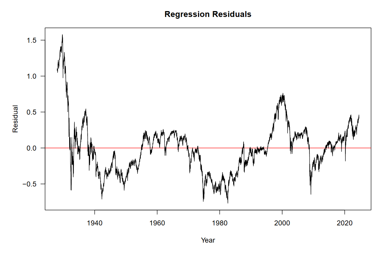
Basically, this is the information “left over” from the model that we still need to explain. I don’t know about you, but I see a sine-wave in the residuals. Generally higher around 1930, the 1960s, 2000, and now. Generally lower around the early 1940s, 1980, and 2009.
Can we find a sine-wave that fits our residuals?
Generally, a sine wave has an amplitude (A), angular frequency (w), and phase (ϕ). Let’s add those parameters to the model and get the optimizer to fit them.
prm <- list(m = 0.0664,
            b = -126.3,
            A = 0,
            w = 0,
            o = 0)

opt <- optim(prm, function(prm) {
    prm <- as.list(prm)

    # fitting the model
    y_hat <- with(prm, (m * x + b) + (A * sin(w * x + o)))

    # minimizing the sum of squared deviations
    sum((log(y) - y_hat) ^ 2)
})

as.list(opt$par)
I ran the optim function and fed the model parameters back into prm a couple times to get these: m = 0.06658, b = -126.6, A = 0.3345, w = 0.1899, and o = -0.593. Magic!
We can now take a look at our nonlinear regression model on a line chart.
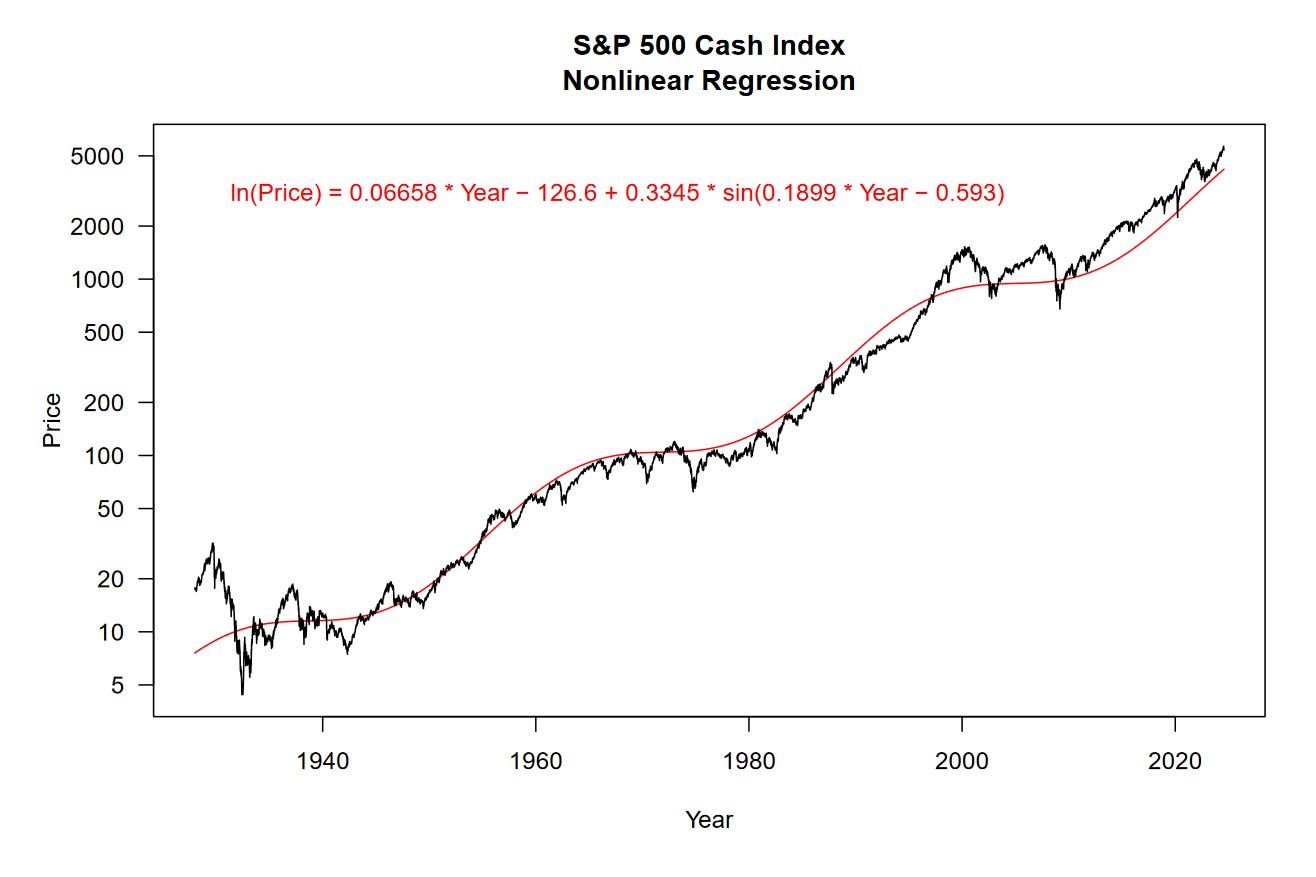
Now we’re wiggling!
The fit of our nonlinear regression is a little better than the previous model, it has an R² value of 97.98% and RMSD of 0.2743. We are explaining more of the variation in the data and we have less total error in the residuals. That’s great.
This is as far as we’ll journey today, there’s plenty here to wrap your head around. The main take away is that by using optimization algorithms, we can fit any equation we can think of in an attempt to explain financial data. If you can understand how to do this for yourself, it is a seriously powerful skill that applies widely.
Before we wrap up, one final curio.
Market Cycles
What if we were to look only at the sine wave component of our model? Perhaps it could tell us something about how the market cycles over a long timeframe.
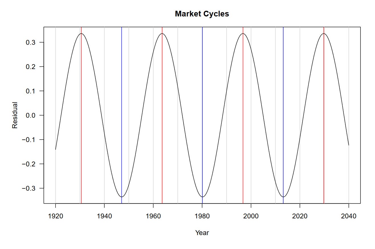
Interesting, it generally agrees with the peaks and troughs we identified.
Be sure to take this chart with a grain of salt. The model we fit is quite rudimentary and we should be careful about extrapolating its results.
That being said, the model predicts that our next major cycle top could be 2030. Previously, my analysis showed that we should reach the $10,000 level on the SPX around that time. Remember that this is from a purely technical context, no fundamentals of investing are considered.
We’ll have to stick around to find out!
Resources
Technical Appendix
The code examples above won’t work unless you have the mysterious yahoo function. For your convenience, all the code necessary to get it working is provided below!
library(dplyr)
library(httr)
library(lubridate)

CGI_YAHOO <- "https://query1.finance.yahoo.com/v7/finance/download/%s?"

concat <- function(...) {
    paste(..., sep = "", collapse = "")
}

clean_names_vec <- function(x) {
    x %>%
        gsub("[^0-9A-Za-z]+", "_", .) %>%
        trimws("both", "_") %>%
        gsub("^(\\d)", "x\\1", .) %>%
        tolower()
}

clean_names <- function(x) {
    names(x) <- names(x) %>%
        clean_names_vec()
    x
}

as_unix_time <- function(date, origin = "1970-01-01") {
    date %>%
        as.POSIXct("UTC", origin = origin) %>%
        as.numeric()
}

api_kwargs <- function(kwargs) {
    paste(names(kwargs), kwargs, sep = "=", collapse = "&")
}

api_format <- function(cgi, kwargs) {
    concat(cgi, api_kwargs(kwargs))
}

api_yahoo <- function(symbol, interval = "1d", events = "history", date0 = "1900-01-01", date1 = today()) {
    kwargs <- c(period1 = as_unix_time(date0),
                period2 = as_unix_time(date1),
                interval = interval,
                events = events)

    CGI_YAHOO %>%
        sprintf(symbol) %>%
        api_format(kwargs)
}

get_yahoo <- function(url) {
    url %>%
        GET() %>%
        content(na = "null") %>%
        clean_names() %>%
        arrange(desc(date))
}

yahoo <- function(symbol, interval = "1d", events = "history", date0 = "1900-01-01", date1 = lubridate::today() + 1) {
    df <- symbol %>%
        api_yahoo(interval, events, date0, date1) %>%
        get_yahoo()

    data.frame(symbol) %>%
        cbind(df) %>%
        as_tibble()
}
If you have issues, email me and we can try to troubleshoot your problem.