

Totally II
The return of market returns.

In this week’s article, we get into shape.
Oh Long Johnson
It has been almost an entire year since I last mentioned Johnson’s SU distribution. This is a real shame because it’s far and away my favorite distribution!

Johnson’s SU is a flexible, unimodal distribution that describes central tendency, variability, skewness, and kurtosis in data. SU stands for “unbounded system,” meaning it is defined over the entire real number line.
If you’re a total nerd like me, read Johnson’s 1949 paper on his systems.
If you are familiar with the normal distribution (“the bell curve”), then you won’t be surprised to know that it only describes central tendency (mean) and variability (standard deviation). Beyond these two parameters, we can also describe skewness, which means the data can favor lower or higher values, making it non-symmetrical. Additionally, kurtosis indicates how prone the data is to extreme values.
The Johnson SU distribution captures all of this variation in parameters, making it a robust yet flexible choice for organic datasets. To truly appreciate what makes Johnson’s SU so powerful, it helps to understand how its flexibility is achieved mathematically. Let’s dive into the nuts and bolts.
Nuts and Bolts
If we take a gander at the cumulative distribution function (CDF) for the Johnson SU, we can begin to understand how this flexibility is possible.
It might look scary at first, but I can break it down for you:
𝑥 is the variable we want to transform.
sinh⁻¹ is the inverse hyperbolic sine (IHS) function.
Φ (phi) is the CDF of the normal distribution.
ξ (xi, pronounced “kzai”) shifts 𝑥 in linear space.
λ (lambda) scales 𝑥 in linear space.
δ (delta) shifts 𝑥 in IHS space.
γ (gamma) scales 𝑥 in IHS space.
Each parameter contributes to shaping the distribution, allowing us to model skewness, kurtosis, and other characteristics of the data in ways that a standard normal distribution cannot.
While it’s tempting to assign a one-to-one correspondence between these four parameters (γ, δ, ξ, λ) and the four properties we want to normalize (skewness, kurtosis, centrality, variability), it’s not technically correct. All four parameters interact to control each property.
For our purposes, we can ignore the CDF of the normal distribution—it’s not relevant to our understanding of the transformation. Instead, we can simplify the description of the Johnson SU CDF into two linear transformations. The first happens in linear space, where ξ shifts 𝑥 and λ scales it. Then, we map from linear space into IHS space and transform again. In this second transformation, δ shifts and γ scales.
A critical feature of the Johnson SU is its use of the inverse hyperbolic sine (IHS) function, which enables it to handle data with a wide range of values, including negative and zero values, in a log-like manner.
Let’s take a look at its formula:
If you’ve worked with data from natural systems, you’ll know how important taking the logarithm (log) of your data can be. This is because exponential series are linearized after taking the logarithm. (I talked about this in an old article.)

What’s frustrating is that we can’t use the log function on negative numbers or zero! The IHS function “solves” this problem. By adding 𝑥 to the square root of the square of 𝑥 plus one, we ensure the range is always positive. Taking the log value of this result allows for a “log-like” mapping for negative, zero, and positive numbers.
See for yourself:
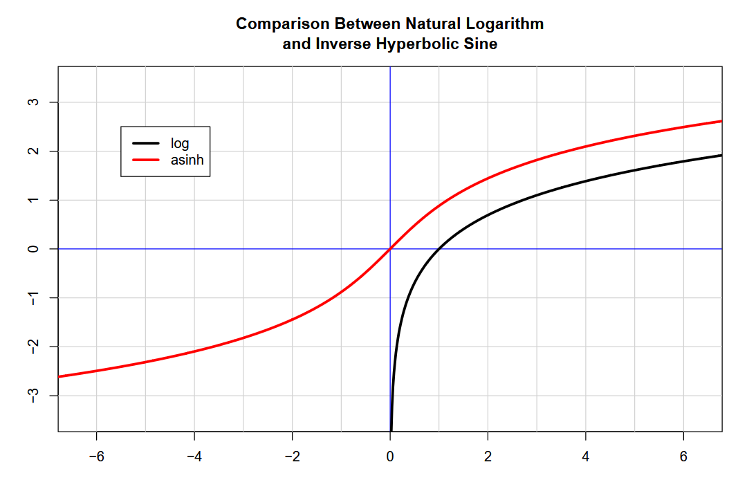
In case you’re wondering, IHS, sinh⁻¹, and asinh all refer to the same function, just in different notations. Notice that the IHS has a variable slope—it is steepest near zero and flattens out in either direction. The parameters of the Johnson SU distribution wiggle this curve to find the “perfect spot” from which to normalize a given distribution, much like how a French curve helps draw a wide variety of contours.
Once we understand the mechanics of the Johnson SU transformation, the next challenge is to fit its parameters to real-world data, but how does that happen?
My Computer is Optimistic
I’ve covered mathematical optimization before on the blog (link below).

To refresh ourselves, mathematical optimization attempts to minimize or maximize the output of a given function. I wish I could fully explain why we use certain functions to fit parameters for a given distribution, but that might take more space than we have now.
Put simply: we minimize the sum of the absolute differences between an actual and theoretical quantile function, then further refine the parameters using the Kolmogorov–Smirnov test.
One last previous article to check out would be the first in this series. Refresh yourself on why we’re trying so hard to accurately model returns from the S&P 500 Total Return index (SPXTR).

Without further ado, here are the results:
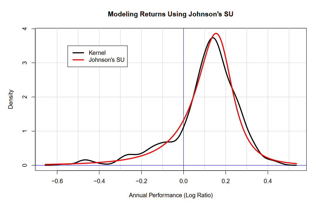
Without a doubt, Nassim Nicholas Taleb would have something to say about the obvious tail risk in markets that the above chart demonstrates. While the most likely result in a given year is a moderate return (our model has a mode of +16.7%), there is a wide variety of outcomes for market returns.
For instance, there’s an 18% chance that returns will be negative for the year. For years with negative returns, the average is -15.9%. For years with positive returns, the average is +18%. The market likes to move. There’s only a 13.6% chance that the return for the year will be between -5% and +5%.
Grains of Salt
Overall, the Johnson SU provides a nuanced and flexible way to model market returns, capturing their variability and tail risks. However, like any model, it is only as reliable as the data it’s based on.
I have to stress that while I believe the Johnson SU distribution adequately captures the nuance of market return distributions, the data is biased to its domain, which spans from 1989 to today.
In the end, the Johnson SU distribution underscores the importance of flexibility in statistical modeling. As markets evolve and datasets grow more complex, tools like these will remain invaluable for making sense of the unpredictable.